Software & Music | Erik Malmqvist Jakobsen

1Introduction

Network theory provides a powerful framework to model relationships and interactions between individuals. With the increasing availability of large-scale, structured datasets from platforms like Spotify, it has become possible to apply network analysis to domains such as music. Viewing artist collaborations through the lens of network science allows us to apply mathematical and computational techniques to analyze which structural properties and patterns they exhibit, and better understand the underlying factors driving their evolution.

Network theory is also a concept with a wide range of use cases, providing a broad abstraction model capable of representing everything from cellular processes and road systems to matchmaking algorithms and social networks. That also means that a problem which has a known solution in one field, surprisingly can lead to answers or insights to questions we have with regards to music collaboration networks that might not initially seem connected. This flexibility gives the opportunity to e.g. explore the evolution of music genre collaborations as a temporal graph or to identify central artists who act as structural bridges across genres or communities.

This study aims to explore the evolution of music collaboration networks over the period 1986 to 2016. Specifically, it seeks to address two main questions: (1) How has the volume and structure of collaboration changed over time? and (2) Which high-collaboration artists can be identified through quantitative network measures? By answering these questions, the project contributes to a better understanding of patterns in artistic collaboration and the roles of individual artists within the network. The following section reviews related work in this area and highlights various approaches to situate the context of this project.

2Related Works

In recent years, numerous studies have investigated music collaboration networks from a variety of perspectives. Depending on the research focus, these networks can be approached through different views and with different goals. Coscia, for example, constructs a network of Italian composers with particular attention to regional background and how geographical closeness influences collaboration ^[1]. Schich et al. take a more historical angle by analyzing the network of British classical composers, focusing on how shared educational backgrounds contribute to community formation and how network position correlates with success ^[2]. Gienapp et al. emphasize genre differences, constructing a case of Jazz and Hip Hop to demonstrate how these different genres lead to distinct network structures and patterns of evolution ^[3]. Meanwhile, Oliveira et al. analyzes how inter-genre collaborations shape both regional and global music markets ^[4].

A methodological challenge is how to model the network itself. In most studies, a music collaboration network is represented as a graph structure, where each node corresponds to an artist, and an edge is added between two artists if they collaborated together. The data itself is embedded as node and edge attributes, such as artist name, genre, and the songs shared between collaborators. When building the graph, one approach, as done by Levy et al. is to begin with a mainstream artist, in this case Drake, and then iteratively expand the network through Drake's collaborators and their collaborators using a Breadth-First Search (BFS) ^[5]. The advantage of this approach is that it quickly leads to an exploration of a dense and influential part of the network. However, this is also its main limitation: it excludes artists who do not collaborate with the chosen starting node or its close neighbors, or artists who do not collaborate at all. Since the starting point is manually selected, this method also potentially introduces sampling bias and may not provide a representative picture of the broader collaboration landscape. To avoid this, this project instead constructs a bipartite graph linking artists and songs directly, and then projects it onto an artist-artist collaboration network where edges represent a collaboration, inspired by the work of Park et al. ^[2].

A structural modeling decision to be made, is which fundamental characteristics the graph should have. Let's say, that you wanted to emphasize certain roles of a collaboration, such as an artist contributing to another artists release e.g. as instrumentalist. To capture this asymmetry, you could make an argument for a graph with directed edges as done by Gienapp et al. ^[3]. However since collaborations are typically treated as a symmetric relationship, undirected edges are the most common choice.

Another consideration is the selection of appropriate node and edge attributes for the graph. In music collaboration networks, nodes often carry metadata such as genre, popularity, nationality, or periods of activity ^[1]. Edges, on the other hand, are typically weighted to reflect the intensity of a collaboration, e.g. measured by the number of co-released tracks between two artists. While edge weights can be good to capture collaboration strength, they also constrain the available tools. For example, Park et al. ^[2] uses clustering coefficients to examine the network of western classical composers, which is useful for identifying community structures. However, standard clustering coefficients do not account for edge weights and may not accurately reflect the strength of collaboration in weighted networks. While weighted variants exist ^[6], they are less commonly used.

When working with these kinds of networks, a commonly used concept is the giant component. The giant component refers to the largest connected subgraph in which any two nodes are connected by a path, and serves as a measure to understand the overall connectivity of a network. It has been used to study the evolution of collaboration networks over time, showing that the size of the giant component grows in proportion to the total number of nodes ^[7], which suggests that the network becomes more connected as more collaborators join.

Another concept in network analysis is centrality — in particular, betweenness centrality, which quantifies how often a node appears on the shortest paths between all pairs of nodes in the network. As a metric, betweenness centrality can highlight artists who act as bridges across genre or community boundaries, facilitating connections between otherwise separate groups of artists. In the context of research citation networks, Leydesdorff demonstrates that betweenness centrality can serve as an indicator of interdisciplinarity, as it reflects an journals role in linking multiple fields ^[8]. In a music setting, this translates to artists who bridge otherwise separate communities or genre clusters. From a computational perspective, the calculation of betweenness centrality is resource-heavy, particularly in large-scale graphs. One of the well known solutions, is Brandes' algorithm that provides an efficient approach for exact computation ^[9], but later sampling-based methods also exists, offering more scalable approximations for use in larger or dynamic networks ^[10].

Beyond structural metrics, recent work has explored diversity in networks using entropy. Entropy is a concept and metric widely used across fields, from physics to information theory, to have a quantitative measure of the balance between diversity and concentration within a set of entities. Oliveira et al. uses entropy to quantify the interdisciplinarity of scientific publications ^[11], which in a music context would reflect how genre-diverse an artist's collaboration neighborhood is, offering a way to quantify stylistic breadth. The most common way to measure this, is with Shannon Entropy, but other metrics such as the Brillouin index and the Gini coefficient have also been proposed to capture similar notions of diversity, each with their own strengths depending on the underlying data and distribution ^[12].

Building on this body of work, the present study combines network topology, genre classification, and temporal analysis to investigate how collaboration patterns evolve over time. In particular, it emphasizes genre diversity and the structural role of artists, using entropy and centrality metrics to quantify influence.

3Data

3.1Spotify Million Playlist Dataset

The dataset used in this study is based on The Spotify Million Playlist Dataset Challenge ^[13], a publicly available dataset designed to improve music recommendation systems. This dataset consists of one million user-generated playlists collected from Spotify between 2010 and 2017. It was selected for its large size and diverse representation of musical preferences in different time periods and genres. From the playlists, a subset of unique tracks was extracted and additional metadata was acquired by querying the Spotify Web API. In the end, the final processed dataset includes 874762 songs, by 186403 artists. Table 1 presents a sample of the JSON data structure. Each entry is indexed by the track ID and contains the specified fields, with artists represented as a nested object.

It is important to acknowledge certain limitations in the dataset. First, the data is inherently biased towards user-generated playlists, meaning that it does not fully represent all music available on Spotify. Additionally, the popularity scores fluctuate over time, since it has emphasis on recent listening trends. The dataset will only capture a snapshot in time, meaning that values may have changed since data collection. Finally, Spotify's genre annotation is by no means complete, and some tracks may lack assigned genres or be misclassified.

Another important limitation concerns the inconsistency of metadata. While the project aims to study collaborations among active or contemporary artists, the dataset includes many releases by classical composers who deceased centuries ago, but whose works continue to be featured in modern playlists. To mitigate this, the 25 most popular classical composers according to Pentreath were excluded from the data ^[15]. Additionally, releases involving more than five credited artists were filtered out, as these often represent compilation albums or highly aggregated credits that can introduce artificial noise in the network. These factors should be considered when interpreting the results.

Track ID	29OaX99VkV4vLX2ab5sKrJ
Track Name	Money On The Floor
Album Name	Live From The Underground
Release Year	2012
Duration (ms)	247160
Popularity	41
Explicit	True
Artists	Big K.R.I.T., 8Ball & MJG, 2 Chainz
Genres	Rap, Southern Hip Hop, Crunk, Memphis Rap

Table 1 — Sample data structure. The popularity score is an algorithmically determined metric provided by Spotify ^[14].

3.2Music Collaboration Graph

With the dataset, I am ready to define a music collaboration graph. As explored by Arram Bae et al. ^[2] by modeling the British composer network, the complete list of song data can naturally be represented as a bipartite graph with two node classes, V_S and V_A. V_S consists of the songs and V_A represents the artists from the dataset. There exists one or more edges from v_S ∈ V_S to artists v_A ∈ V_A, if v_A was credited in the song's metadata.

Figure 1 — bipartite network of songs and artists, and its one-mode projection onto artists — Figure 1 — (a) Bipartite network of the songs and artists. (b) One-mode projection of the bipartite network onto the set of artists by connecting artists when they are associated with a common release. Edge weights equal the number of releases they did together.

To derive the yearly collaboration networks, I project this bipartite graph onto the artist node set. Specifically, for each year t, I form an undirected edge (u, v) ∈ E_t between two artists u and v if they both contributed to at least one song released in year t. Figure 1 illustrates an example of the graph creating process.

With the artist-to-artist projection, the temporal music collaboration network is then modeled as a sequence of undirected graphs

G = {G₁₉₈₆, G₁₉₈₇, . . . , G₂₀₁₆},

where each single snapshot G_t = (V_t, E_t) represents the state of the collaboration network in year t. This means the model is not accumulative or overlapping between years, but reflects discrete yearly views of the network, as described by Coscia ^[16].

The set of vertices V_t consists of all artists who released at least one record in year t. The set of undirected edges E_t ⊆ V_t × V_t captures collaborations between artists during the same year.

An edge (u, v) ∈ E_t exists if artists u and v collaborated on at least one release in year t. Each edge is assigned a weight w_t(u, v) ∈ ℕ, representing the number of joint releases by u and v in that year.

3.2.1Genres

Each node and edge in G_t is annotated with genre information derived from the songs of the dataset. For artist nodes, this takes the form of (1) one single primary genre, and (2) a multiset of genres representing all genre labels from the songs the artist participated in during year t, allowing for repeated occurrences of the same genre. Similarly, each edge (u, v) ∈ E_t stores a multiset of genres corresponding to all collaborative tracks between artists u and v in that year.

From the 673 unique present genres, each artist node is assigned a single primary genre. The motivation for this, is to abstract some of the complexity away and facilitate some more general comparisons across years and genres.

To derive these primary genres, all genre labels were manually grouped into a set of nine supergenres (e.g., Pop, Rock, Hip Hop, etc.). This mapping process was done manually by personal judgment, but I will discuss alternative approaches in the later sections. The distribution among the frequencies of genre appearing in the data, and which super-genre they belong too, are visualized as a tree-map in Appendix 8.1. Once each genre was assigned to a super-genre, the primary genre of a node was determined by a simple majority vote over the node's genre multiset for a given year. In cases of ties, one of the top supergenres was selected at random.

4Methodology

These sections outline the methodological approaches taken, and how they are implemented in this project from the context of the related works.

4.1Giant Component

To understand the overall connectivity of music collaborations, this study examines the giant component in yearly snapshots of the network. The giant component is the largest connected subgraph, commonly used to assess whether a network is cohesive or fragmented. In this context, its growth over time is interpreted as a sign of increasing connectivity and broader access to collaboration opportunities. The size of the giant component serves as a tool to understand how centralized or diffuse the collaboration network is in a given year.

4.2Degree Distribution and Power-Law Exponents

Degree distributions are analyzed for both the full collaboration graph and its giant component, across each year from 1986 to 2016. For each case, the distribution is fitted to a power-law model of the form

P(k) ∼ k^−α

Where k is the degree and α is the scaling exponent. The exponent α is estimated using maximum likelihood estimation (MLE), which identifies the value that best fits the observed degree distribution. This is done with the python package powerlaw ^[17]. A lower value of α indicates a heavier tail, meaning that a small number of artists maintain a high number of collaborations, which is typical for scale-free networks. Comparing these values over time provides insight into how collaborations are distributed across the network, whether they remain concentrated among a few central artists or becomes more evenly spread. This also allows us to assess whether the network maintains scale-free characteristics as it evolves.

4.3Betweenness Centrality

Betweenness centrality is a widely used measure for identifying nodes that serve as bridges or intermediaries within a network. For a given artist, the betweenness centrality score reflects the number of shortest paths between all other pairs of artists that pass through that artist. High betweenness indicates that an artist plays a crucial role in connecting different parts of the network, potentially bridging otherwise disconnected groups or distant parts of the network.

The formal definition of betweenness centrality, is defined as

C_B(v) = Σs,t∈Vσ(s, t|v)σ(s, t)

where σ(s, t) is the number of shortest paths between nodes s and t, and σ(s, t|v) is the number of those paths that pass through node v.

If s = t, then σ(s, t) = 1. If v ∈ {s, t}, then σ(s, t | v) = 0, since a node is not considered to lie on a path between itself and another node.

In this study, edge weights are not considered and all collaborations are treated equally. This means that the shortest path distances are computed purely on the basis of the number of edges and not their strength.

Betweenness centrality is computed annually for all nodes in the collaboration graph from 1986 to 2016. In later years, as the network grows larger and exact computation becomes increasingly resource-intensive, an approximation method is used to estimate scores more efficiently. While these approximations may not yield precise values, they preserve the relative ordering of nodes. Meaning that artists with higher centrality still rank above those with lower centrality. These scores help highlight artists who occupy central structural positions in the network.

4.4Entropy

Entropy is used here to measure the diversity of genres in an artist's collaboration neighborhood. A higher entropy score, will suggest that an artist collaborates more broadly across genres, and a lower score suggests that artists are more likely to collaborate within the same genres.

To compute an artist's entropy value, I take the same approach as Silva et al. ^[11]. I construct the histogram h_a(g), representing the frequency of each genre g appearing among the artists connected to artist a. As described in 3.2, genre labels from these artists are appended to the artist's genre attribute when constructing the graph, allowing duplicates, meaning that genres can contribute multiple times based on the number of collaborations. This also makes edge weights redundant in this case, as including them would introduce the problem of having genre counts scale artificially with the number of collaborators per release.

To avoid the entropy measure being dominated by the most frequent genre labels, each histogram h_a(g) is normalized by dividing by the global frequency of genre g throughout the entire network:

h̄_a(g) = h_a(g)Σ_j h_j(g)

The normalized values h̄_a(g) are then transformed into a probability distribution P_a(g):

P_a(g) = h̄_a(g)Σ_g′ h̄_a(g′)

Finally, the entropy is computed as:

H_a = −ΣgP_a(g) · log P_a(g)

One of the limitations of this approach is that it does not consider the closeness or relationship between genres, and therefore does not account for semantic or stylistic similarity. Shannon entropy does not capture the natural hierarchical structure of genre labels. For example, Shannon entropy treats synth pop and pop as equally distinct as heavy metal and christmas, even though the former are more closely related. As such, while entropy gives a useful indication of variety, it does not directly reflect genre distance or blending across genre hierarchical trees.

5Results and Analysis

5.1Graph Summary

As a foundation for examining the evolution of the network, Table 2 provides a yearly overview of the graph snapshots from 1986 to 2016. For each year, the total number of artist nodes and collaboration edges are listed, along with giant component (GC), including its size and average degree.

Year	Nodes	Edges	GC Nodes	GC Edges	Avg. Degree	GC Avg. Degree	Collab %
1986	932	318	30	51	0.682	3.400	11.41
1987	1,175	619	64	106	1.054	3.312	14.48
1988	1,330	708	58	95	1.065	3.276	16.02
1989	1,340	591	58	100	0.882	3.448	13.13
1990	1,808	923	157	279	1.021	3.554	16.16
1991	1,855	924	52	97	0.996	3.731	13.66
1992	1,986	932	135	256	0.939	3.793	13.22
1993	2,226	906	91	168	0.814	3.692	11.10
1994	2,664	1,376	267	471	1.033	3.528	13.84
1995	2,821	1,303	182	326	0.924	3.582	14.36
1996	3,064	1,418	71	127	0.926	3.577	13.01
1997	3,315	1,601	182	340	0.966	3.736	13.95
1998	3,648	2,072	337	643	1.136	3.816	15.63
1999	4,239	2,435	452	784	1.149	3.469	15.99
2000	4,666	2,440	412	720	1.046	3.495	15.97
2001	4,845	2,473	352	686	1.021	3.898	12.74
2002	5,060	2,417	449	755	0.955	3.363	12.71
2003	5,825	2,758	649	1,141	0.947	3.516	13.55
2004	6,297	2,840	487	887	0.902	3.643	12.83
2005	8,086	3,605	748	1,310	0.892	3.503	13.15
2006	9,646	4,332	977	1,794	0.898	3.672	13.32
2007	10,549	4,528	1,058	1,830	0.858	3.459	13.41
2008	11,955	4,884	797	1,422	0.817	3.568	12.07
2009	14,574	6,348	1,312	2,238	0.871	3.412	13.66
2010	17,738	7,902	1,839	3,197	0.891	3.477	13.77
2011	21,715	10,608	2,966	5,146	0.977	3.470	15.06
2012	25,412	14,748	4,416	7,804	1.161	3.534	18.05
2013	28,092	16,985	5,526	9,794	1.209	3.545	18.74
2014	31,562	20,256	7,007	12,129	1.284	3.462	21.16
2015	35,293	24,968	9,209	16,504	1.415	3.584	23.47
2016	39,085	29,708	11,723	20,987	1.520	3.580	25.67

Table 2 — Graph summary of the collaboration network. The collaboration percentages are the share of nodes from the bipartite graph with degree greater than one, or simply the songs, with more than one credited artist.

The collaboration percentage represents the proportion of songs in each year that were created by more than one credited artist. In the bipartite graph, this corresponds to the share of song nodes with a degree greater than one. Interestingly, while the collaboration percentage increases significantly over time, from around 11% in the late 1980s to over 25% by 2016—the average degree of the artist nodes grows at a much slower rate. This suggests that although collaborations became more common, they did not necessarily lead to a denser network of artist relationships. One possible explanation is, that collaborative songs are released by the same highly active artists, which inflates the collaboration percentage, as these primarily reinforces existing links without increasing the average number of distinct co-collaborators per artist.

Another interpretation of this, is that while collaboration frequency increases, but the average degree does not grow at the same pace, could be because the artists collaborate more frequently but with the same kind of artists rather than different ones.

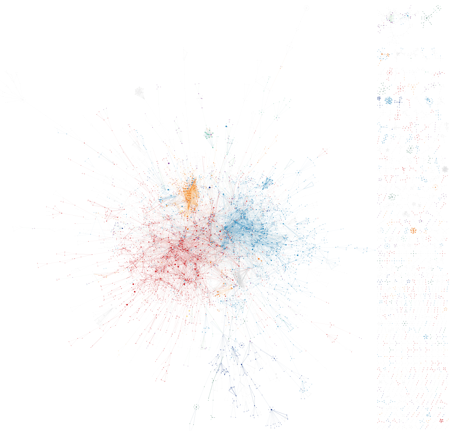
Fig. 2 presents a snapshot of the collaboration network in 2016, highlighting the giant component alongside the smaller disconnected subcomponents. The giant component dominates the network and connects the majority of active artists.

5.2Degree Distribution

To explore this idea further, I examined the degree distribution of the collaboration network over time. Fig. 3 and Fig. 4 shows a plot of the frequencies of degrees for artists over the years. The degree distribution for both the full network and the giant components shows a pattern that, some artists are super collaborators while the majority has very few collaborations. This pattern is typical for social networks, which exhibits scale-free properties.

Figure 3 — log-log plot of the artists' degree distributions over years — Figure 3 — Log-Log plot of the artists' degree distributions over years.

Figure 4 — log-log plot of the artists' degree distribution in the giant component over years — Figure 4 — Log-Log plot of the artists degree distribution in the giant component over years.

The power-law exponent α was computed for both the full graph and its giant component each year. As shown in Figure 5, the values of α fluctuate considerably in the early years but gradually stabilize from the late 1990s onward.

High values of α, in particular 1990 and 1993, suggest a network with very few super-collaborators and degrees more evenly spread. These spikes possibly reflect sparsity in the early data, where fewer collaborations are recorded and the network is still fragmented, but could also indicate the presence of disconnected subgroups or more local music communities that had not yet integrated into the giant component.

Figure 5 — power-law exponents of the yearly snapshots in the full graph and the giant component, 1986–2016 — Figure 5 — The power-law exponents of the yearly snapshots in the full graph and and the giant components.

As the network matures, α values converge toward a range between 3 and 4. This indicates a more classic structure, that a small number of artists are highly connected, while the majority maintain few connections. These lower α values correspond to heavier-tailed distributions, typical of social and collaboration networks where hubs emerge over time.

One possible interpretation of the convergence between the power-law exponents of the full graph and the giant component is that the overall music collaboration network has become more integrated over time. As the network evolves, more artists appear to join the giant component, meaning their collaborations now link them into the broader, shared network. This could potentially reflect a general trend in the music industry, that the rise of global platforms like Spotify have contributed in facilitating collaborations, making it easier to co-release songs.

5.3Genre Evolution

Figure 6 shows the evolution of mean betweenness centrality scores by genre from 1996 to 2016. Two key patterns stand out. First, genres like hip-hop and r&b consistently rank higher than others, particularly from the early 2000s onward. This suggests that artists in these genres frequently act as bridges or as facilitators of collaborating within the network. Their central structural role may reflect a more collaborative culture of these genres. On the other hand, genres like classical, country, and folk-world remain consistently lower in betweenness centrality. These genres may be more self-contained, with fewer collaborations in general, or less represented in global digital platforms.

Secondly, there is a general upward trend in mean betweenness centrality scores across most genres throughout the time period. This could indicate, that some artists are increasingly occupying structurally important positions. This can happen when the network relies more heavily on specific individuals to link otherwise separate parts of the graph together.

Figure 6 — mean betweenness centrality of the different main genres throughout the years — Figure 6 — Mean betweenness centrality of the different main genres throughout the years.

In summary, although collaboration frequency increases over time, as shown by the rising collaboration percentage, this does not result in a proportionate rise in average degree. This suggests that while artists are collaborating more, they often do so within familiar circles, reinforcing existing relationships rather than forming new ones.

At the same time, the growth of the giant component and the convergence of the power-law exponent indicate that the network is becoming more globally integrated. More artists are connected to the broader network, but the mean betweenness centrality suggests that smaller number of them take on increasingly important roles in holding the network together.

So while the network as a whole may not be significantly denser in terms of local connections per artist, it is becoming more structurally centralized, with collaboration more facilitated through key artists who act as bridges. This reflects a shift toward a more hierarchical structure, where a few highly connected artists serve as access points between otherwise distinct groups of artists.

5.4High Collaboration Artists

This section highlights the most prominent collaborators in the network, identified through high scores in both entropy and betweenness centrality. Appendix 8.2 provides a year-by-year overview of the top 10 artists for each metric. Several artists stood out by ranking in the top 10 for both measures in the same year — indicating not only a high degree of stylistic diversity in their collaborations but also a structurally central position in the network. Those who were among the top 10 artists in both measures include Donald Fraser and Berliner Philharmoniker (1996), JAY-Z (1998), Xzibit (2000), Jadakiss and Diddy (2001), Linkin Park (2002), Snoop Dogg (2006), Akon (2008), Busta Rhymes and Lil Wayne (2009), Pitbull (2010), Tiësto (2012), Dido and French Montana (2013), Yellow Claw (2015), Ty Dolla $ign and French Montana (2016).

Some artists appeared in the top 10 across multiple decades, showing a long-term presence in music collaborations. Among all, Snoop Dogg had the most total appearances, showing up 14 times between 2000 and 2016. Close behind was Indian film composer A.R. Rahman, who appeared 12 times from 1999 to 2016. Figure 7 visualizes the two-hop collaboration network centered around Snoop Dogg in 2011. Edge and node colors represents the different main genres of Snoop Dogg's neighborhood.

Figure 7 — two-hop collaboration network centered on Snoop Dogg in 2011 — Figure 7 — Two-hop collaboration network centered on Snoop Dogg in 2011. Appendix 8.3 has a full size version with artist labels.

A few others also stood out for their decade-spanning relevance. Shankar Mahadevan and the trio Shankar-Ehsaan-Loy related to the scene of Indian soundtrack, appeared in the early 2000s and showed up again in later years. Ludacris made it to the list in the early 2000s and again in the mid-2010s, pointing to a career with sustaining impact. While artists like Too $hort only show up a couple of times, they still span a wide time range, hinting at a lasting, if more occasional, impact on the collaboration scene.

6Discussion

In this discussion, I will reflect on how the results can be interpreted, consider alternative approaches that could have been taken, address limitations and what did not go as planned.

To answer how the structure and volume of collaborations has changed throughout the years, the results show, that collaborations in music have increased significantly over the 30-year period studied. The raw collaboration percentage rose from around 11% in 1986 to over 25% in 2016. However, the average degree for artists did not grow nearly as much, which suggests that while more collaborations are happening, they often take place within the same circles. It might have been helpful to include edge weights in this part of the analysis, as they were in the end not used at all. These could potentially have helped explain, why the overall percentage of collaborations increase but the distinct collaborators of an artist does not.

The growing size of the giant component further indicates that more artists are becoming part of a shared, interconnected collaboration space. Combined with the convergence of power-law exponents between the full graph and the giant component, this suggests that the network is becoming more globally integrated. At the same time, the average betweenness centrality is increasing across nearly all genres. This could indicate that integration is not happening evenly, but rather through a smaller number of key artists who act as bridges between different groups or clusters. The network does not seem to become uniformly denser, instead, it is becoming more structurally centralized around influential artists.

Entropy was used in this project to quantify how genre-diverse an artist's collaboration neighborhood is, and how stylistically broad their connections are. While this gives some insight at the individual artist level, it's still fair to question how well this approach actually works in this context.

Figure 8 — entropy distribution of the period 1996 to 2016 — Figure 8 — Entropy distribution of the period 1996 to 2016.

Figure 9 — a null model with randomized genres on the nodes — Figure 9 — A null model with randomized genres on the nodes.

To investigate this, entropy was calculated on the full network — not as yearly snapshots, in order to get a larger and more stable dataset. Figure 8 shows the distribution of entropy scores for all artists across the full period. The idea to use entropy in this way is inspired by Silva et al. ^[11], who applied it in academic citation networks to measure the interdisciplinarity of journals. Based on that, I had hoped the distribution would follow a power-law shape, similar to how degree distributions often do in network analysis.

However, the resulting entropy distribution showed clear plateaus, especially around values at 0.69, 1.11, and 1.60. These correspond to log-based values of 1, 2, and 3, which makes sense, since many low-degree artists in the dataset are only annotated with one, two, or three genres. To check whether the entropy calculations themselves were working correctly, Figure 9 shows a null model, where the number of genres per artist was kept the same, but the genres were randomly shuffled across nodes.

The null model shows plateaus around the same values as the actual distribution, but overall follows a smoother curve, more in line with what you would expect from randomized data. This suggests that the entropy was calculated correctly. However, it also suggests that the entropy measure is less effective in this dataset than hoped, mainly because many artists simply do not have enough genre labels to produce a meaningful spread. In contrast, the citation networks studied by Silva et al. ^[11] involve hundreds of citations per journal, which provides much richer data to work with. Here, the relatively small number of genre annotations per artist limits how much insight entropy can provide on its own.

Despite these issues, ranking artists by betweenness centrality and entropy ended up highlighting several well-known artists, for example, Snoop Dogg and JAY-Z. So even though there were some challenges with how well the chosen metrics capture diversity or bridge-building roles, it is still satisfying to see artists like these stand out in the results. Both can be argued to have played major roles in shaping the mainstream music scene and have had careers marked by genre shifts and collaborations across musical boundaries.

6.1Limitations

One important discussion point concerns the dataset itself, which presented several challenges from the beginning due to inconsistent metadata. For example, classical composers were filtered out during preprocessing, as they are long deceased and their inclusion introduced noise in the data. Despite these efforts, a significant amount of unintended content remains. In particular, aggregated Spotify profiles such as Various Artists or Traditional caused problems. These profiles often have millions of monthly listeners and scored highly on metrics like entropy and betweenness centrality, even though they don't represent a single, real artist, but rather a collection of different contributors. In such cases, it was difficult to identify the actual artist behind a release, which made the interpretation of results more complicated.

Beyond the metadata itself, the size and balance of the dataset across time also raise questions. The earliest years, especially from 1986 to 1996, are heavily underrepresented compared to later periods. This makes it difficult to assess whether patterns observed in those early years, such as spikes or drops in average degree or power-law exponents, reflect real structural properties or are simply due to limited data. Similarly, as the dataset grows larger in the 2000s and 2010s, it becomes harder to say whether the convergence of metrics like the power-law coefficient is driven by actual changes in the collaboration network or just the effect of more data smoothing out variation.

Another limitation relates to how genres were handled. In this project, all genre labels were manually grouped into a smaller set of supergenres based on my personal judgment. But what qualifies as a supergenre is subjective, and the grouping process could have been more robust. One solution could be, to have queried an external service for assistance. For example, McDonald has developed a tool that, for each Spotify genre, provides a ranked list of the most similar genres based on audio features and listening patterns ^[18].

The dataset also contained several other fields that could have been interesting to explore. For example, the popularity metric ended up not being used at all, but it could have been relevant to study whether there is a structural connection between collaboration patterns and artist success. It might have been possible to compare how different types of collaboration relate to popularity. Popularity is just one of many data points available through Spotify's API. Other features like tempo, speechiness, energy, and acousticness could also have been used to e.g. classify genres in a more data-driven way, rather than relying only on manual grouping.

Another thing worth discussing is the choice of how the network was modeled over time. In this project, each graph snapshot was built per year, meaning that edges only reflect collaborations that happened within that specific year. While this gives a clean and simple view of the network's evolution, it also means some information is lost, for example, longer-term or repeated collaborations across years are not captured. An alternative approach could have been to model the graph in an accumulative way, where collaborations persist across the years. This or other temporal modeling choices, could especially have brought more insights when analyzing the individual artists collaborations, and in general might have given a different picture of connectivity over time.

In summary, this project shows how network-based metrics can reveal patterns in music collaborations. Despite certain methodological and data-related challenges, the study demonstrates use of network analysis to provides a structured way to examine how artists connect, how collaboration evolves over time, and how roles such as influence and diversity can be quantified, highlighting the value of using network science to understand dynamics of music.

7Conclusion

This project set out to examine the evolution and structure of music collaboration networks from 1986 to 2016 by modeling artist relationships as a temporal graph. Through a combination of structural metrics, such as degree distribution, giant component size and power-law exponents, as well as node-oriented measures such as betweenness centrality and entropy, the analysis provided insight into how collaboration patterns have changed over time.

The results show that the network has become increasingly connected, with more artists joining the giant component and overall collaboration frequency rising. However, this growth has not translated into a uniformly denser network. Instead, the results suggest a shift toward greater structural centralization, where a smaller number of highly connected artists play a key role in holding the network together. Betweenness centrality suggests the emergence of such bridge-building artists, particularly in genres like Hip-Hop and R&B.

Inspired by similar uses of entropy in interdisciplinary research, entropy was here used to explore genre diversity in collaborations of artists. When paired with centrality, it helped identify artists with both stylistic breadth and structural importance.

Overall, this study demonstrates how network science can offer valuable perspectives on artistic collaboration and genre dynamics in musical collaboration networks. While some limitations, especially around data quality and genre handling affected the insights, the project still provides a meaningful approach to studying structural and temporal patterns in music collaboration networks. Network metrics are shown to be useful for reasoning about artists influence, connectivity, and diversity, and they help frame music not only as an artistic product but as a connected, evolving system shaped by patterns of collaboration.

References

[1]Michele Coscia. Node Attribute Analysis for Cultural Data Analytics: A Case Study on Italian XX-XXI Century Music. Appl Netw Sci 9, 2024. Link
[2]Maximilian Schich, Juyong Park, Doheum Park, Arram Bae. Topology and evolution of the network of western classical music composers. EPJ Data Science, 2015. Link
[3]Manuel Burghardt, Lukas Gienapp, Clara Kruckenberg. Topological properties of music collaboration networks: The case of Jazz and Hip Hop. Digital Humanities Quarterly, 2021. Link
[4]Danilo B. Seufitelli, Anisio Lacerda, Mirella M. Moro, Gabriel P. Oliveira, Mariana O. Silva. Detecting Collaboration Profiles in Success-Based Music Genre Networks. International Society for Music Information Retrieval, 2020. Link
[5]Vincent Po, Daniel Wood, Erica Wu, Akash Levy, Sunny He. The Musical Collaboration Graph. 2017. Link
[6]Pietro Panzarasa, Tore Opsahl. Clustering in weighted networks, page 155-163. Social Networks 31, 2009. Link
[7]Jörn Grahl, Pascal Budner. Collaboration Networks in the Music Industry. 2016. Link
[8]Loet Leydesdorff. Betweenness as an Indicator of the Interdisciplinarity of Scientific Journals. Journal of the American Society for Information Science and Technology, 2007. Link
[9]Ulrik Brandes. A Faster Algorithm for Betweenness Centrality. 2001. Link
[10]David A. Bader, Shiva Kintali, Kamesh Madduri, Milena Mihail. Approximating Betweenness Centrality. 2007. Link
[11]F.N. Silva, F.A. Rodrigues, O.N. Oliveira Jr, L. da F. Costa. Quantifying the interdisciplinarity of scientific journals and fields, pages 469-477. Journal of Informetrics, Volume 7, Issue 2, 2013. Link
[12]Qi Wang, Jesper Wiborg Schneider. Consistency and validity of interdisciplinarity measures. 2020. Link
[13]Spotify, Johannes Kepler University, The University of Massachusetts. Spotify Million Playlist Dataset Challenge. Spotify, 2020. Link
[14]Spotify. Spotify Web API. Spotify, 2025. Link
[15]Rosie Pentreath. The 30 greatest classical music composers of all time. Classic.fm, 2020. Link
[16]Michele Coscia. The Atlas for the Aspiring Network Scientist, page 114. 2025. Link
[17]Jeff Alstott, Ed Bullmore, Dietmar Plenz. powerlaw: A Python Package for Analysis of Heavy-Tailed Distributions. 2014. Link
[18]Glenn McDonald. Every Noise at Once. 2025. Link

8Appendix

BA_erja.pdf

8.1Super-Genre Tree Map Plot

Tree map of the 673 unique genres grouped into nine supergenres, sized by frequency — Distribution of the 673 unique genres present in the data, grouped into nine supergenres and sized by frequency.

8.2Top 10 Scoring Artists

Table 3 — Top 10 artists ranked by betweenness centrality and entropy, for every year from 1996 to 2016.

View Table 3

8.32-Hop Neighborhood

Figure 11 — two-hop collaboration network centered on Snoop Dogg in 2011, with artist labels — Figure 11 — Two-hop collaboration network centered on Snoop Dogg in 2011. Node sizes reflect degree; edge thickness represents collaboration weight; node colors indicate genre.